Equation of State
Introduction
Depending on how you solve the TOV equation, which describes a non-rotating neutron star (NS) in hydrostatic equilibrium, you will end up with different NS parameters. The nominal two parameters used to illustrate differences in equation of state (EOS) are mass and radius.
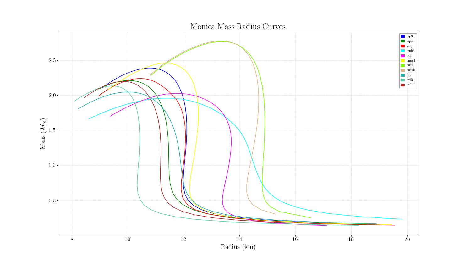
Mass-Radius Curves
For a subset of EOSs, we can plot mass radius curves.
>>> from distutils.spawn import find_executable
>>> from gwemlightcurves.KNModels import table
>>> from gwpy.table import EventTable
>>> from gwpy.plotter import EventTablePlot
>>> plot = EventTablePlot(figsize=(18.5, 10.5))
>>> ax = plot.gca()
>>> EOS = ['ap3', 'ap4', 'eng', 'gnh3', 'H4', 'mpa1', 'ms1', 'ms1b', 'sly', 'wff1', 'wff2']
>>> Color = ['blue', 'green', 'red', 'cyan', 'magenta', 'yellow', 'chartreuse', 'burlywood', 'lightseagreen', 'mediumaquamarine', 'brown']
>>> EOS_Color = dict(zip(EOS, Color))
>>> for eos in EOS:
>>>     t=EventTable.read(find_executable(eos+'_mr.dat'), format='ascii')
>>>     mask=t['radius']<20
>>>     ax.plot(t['radius'][mask], t['mass'][mask], color=EOS_Color[eos], label=eos)
>>> ax.set_xlabel("Radius (km)")
>>> ax.set_ylabel("Mass ($M_{\odot}$)")
>>> ax.set_title('Monica Mass Radius Curves')
>>> plot.add_legend()
(Source code, png, hires.png, pdf)

Maximum NS Mass
Each equation of state has a maximum allowed mass. This, along with several other constraints arising from causality and limitations on spin, determine what masses and radii are allowed for NSs.
EOS From Polytropes
LALSimulation also has the capability to construct an EOS using a set of 4 polytrope parameters, as in Read et al.
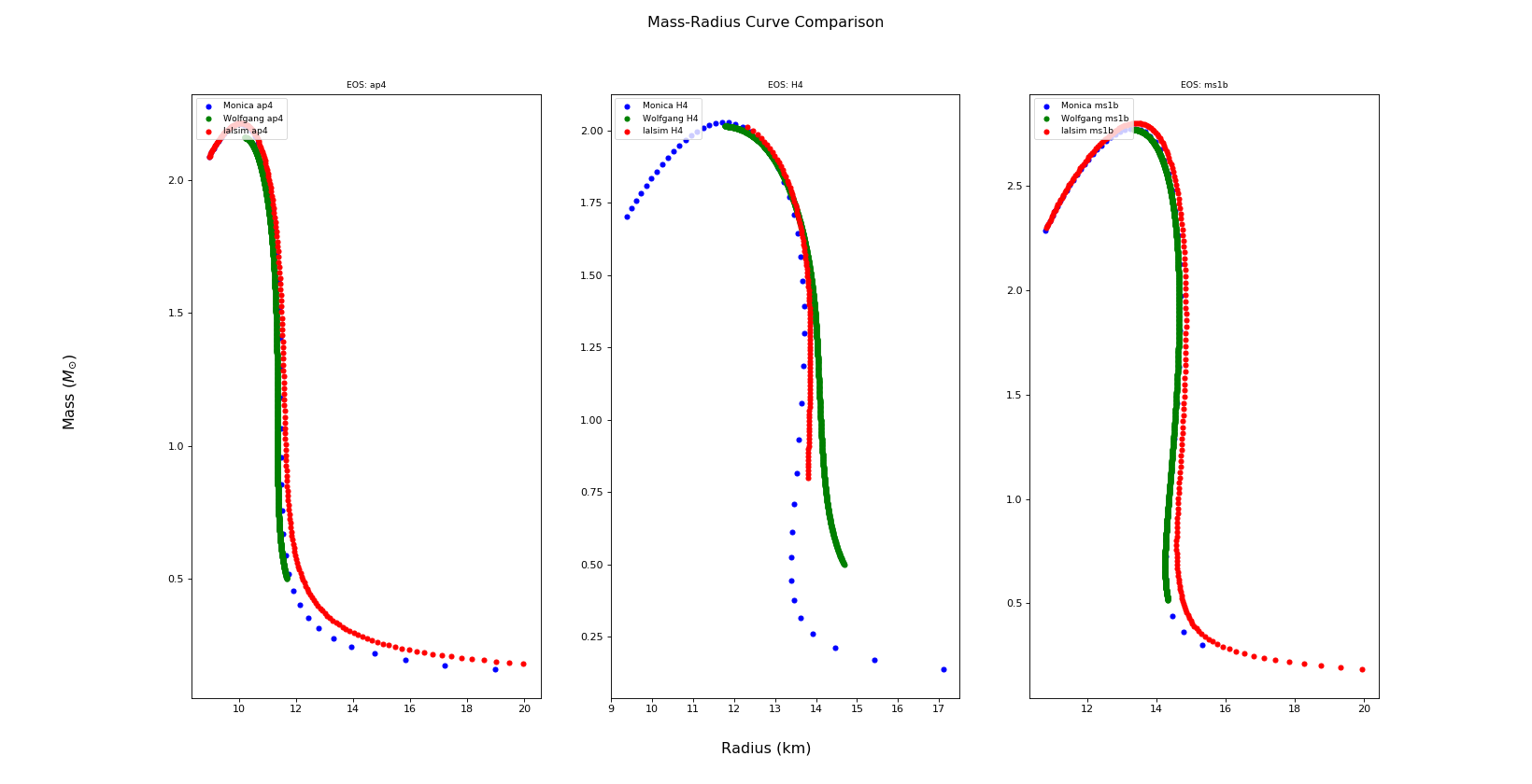
Direct Comparison
Here we plot a direct comparison of mass radius curves from the three different TOV solvers.
>>> from distutils.spawn import find_executable
>>> from gwemlightcurves.KNModels import table
>>> from gwpy.table import EventTable
>>> from gwpy.plotter import EventTablePlot
>>> import astropy.units as u
>>> import astropy.constants as C
>>> G = C.G.value; c = C.c.value; msun = u.M_sun.to(u.kg)
>>> plot = EventTablePlot(figsize=(20.5, 10.5))
>>> EOS = ['ap4', 'H4', 'ms1b']
>>> Color = ['blue', 'green', 'red']
>>> locations = [(1,3,1), (1,3,2), (1,3,3)]
>>> plot_location = dict(zip(EOS, locations))
>>> for eos in EOS:
>>>     ax = plot.add_subplot(plot_location[eos][0], plot_location[eos][1], plot_location[eos][2])
>>>     ax.set_title('EOS: {0}'.format(eos), fontsize='small')
>>>     t_mon=EventTable.read(find_executable(eos+'_mr.dat'), format='ascii')
>>>     t_wk=EventTable.read(find_executable(eos+'.tidal.seq'), format='ascii')
>>>     t_lalsim=EventTable.read(find_executable(eos+'_lalsim_mr.dat'), format='ascii')
>>>     wk_conversion=(msun * G / c**2)*10**-3
>>>     mask_mon=t_mon['radius']<20
>>>     mask_wk=t_wk['Circumferential_radius']<20
>>>     mask_lalsim=t_lalsim['radius']<20
>>>     plot.add_scatter(t_mon['radius'][mask_mon], t_mon['mass'][mask_mon], label='Monica '+eos ,color=Color[0], ax=ax)
>>>     plot.add_scatter(t_wk['Circumferential_radius'][mask_wk]*wk_conversion, t_wk['grav_mass'][mask_wk], label='Wolfgang '+eos ,color=Color[1], ax=ax)
>>>     plot.add_scatter(t_lalsim['radius'][mask_lalsim], t_lalsim['mass'][mask_lalsim], label='lalsim '+eos ,color=Color[2], ax=ax)
>>>     plot.add_legend(loc="upper left", fancybox=True, fontsize='small')
>>> plot.text(0.5, 0.04, 'Radius (km)', ha='center', fontsize='x-large')
>>> plot.text(0.04, 0.5, 'Mass ($M_{\odot}$)', va='center', rotation='vertical', fontsize='x-large')
>>> plot.suptitle('Mass-Radius Curve Comparison', fontsize='x-large')
(Source code, png, hires.png, pdf)