Simulating a Kilonova Lightcurve
Introduction
When attempting to simulate the lightcurve froma kilonova assosciated with a binary coalesence, a number of parameters must be determine first. First of all, is the system a binary neutron star system or a neutron star black hole system. This determination will effect which fit model you utilize in order to calculate the expected dynamical ejecta mass (and velocity) that arises from the system. For binary neutron stars, one can use Tim Dietrich and Maximiliano Ujevic, and for a NSBH one can use Kawaguchi. These fits tie information such as compactness, baryonic mass, and mass of the objects to the expected ejecta. These fits come with uncertainities of ~72% but knowing the ejecta mass is critical when determining the expected lightcurve from the resulting kilonova. We now explain how one can go froma set of posteriors of the system to generating the expected lightcurve from the kilonova. We consider many important things including whether or not you make Equation of State (EOS) assumptions. Whether or not you use fits for compactness and baryonic mass and how you treat the uncertainity in ejecta that comes with the fit.
Reading and using KNTable
The KNTable object comes with a read_samples(), allowing
trivial reading of samples:
>>> from gwemlightcurves.KNModels import KNTable
>>> t = KNTable.read_samples('posterior_samples.dat')
The results should look like this:
>>> print(t)
   dlambdat     costheta_jn   ...      dec       matched_filter_snr
-------------- -------------- ... -------------- ------------------
-424.431604646 0.848696760069 ... 0.577824127959      33.5477773932
-147.120517819 0.991997169733 ... 0.576384671836      33.5566982929
-240.912505017 0.976047933498 ... 0.577896147804      33.6263488512
-186.290687306 0.727047513491 ... 0.582878134524      33.4518918366
-210.457602464 0.967621722464 ... 0.580780890411      33.5696948608
0.377168713485 0.653066039319 ...  0.57000694353      33.5307165083
-350.294734561 0.891785128102 ... 0.585910104721      33.5685077643
           ...            ... ...            ...                ...
-37.5863972893 0.975612607455 ... 0.575280574082      33.6140080488
-128.526058992 0.698513990317 ... 0.581271675244      33.5713366289
-10.3419873355 0.971274339543 ... 0.576536076406      33.6291236021
 202.992550229 0.967479803846 ... 0.571265399682      33.5992585584
-21.5943515138 0.673295017122 ... 0.578523325358      33.3765394973
 82.6149783838 0.941362067895 ... 0.582807999184      33.5504875571
 -490.19334394  0.83602530718 ... 0.564811075217      33.6087938033
Length = 1996 rows
After loading the table, one can caluclate lambda1 and lambda2 from dtilde if it is not already in the samples.
calc_tidal_lambda():
>>> t = t.calc_tidal_lambda(remove_negative_lambda=True)
After accomplishing the reading of the sample, let’s say we want to calculate
compactness from radius. This would require calculating the radius from a mass radius curve. We can use gwemlightcurves.KNModels.KNTable.calc_radius(). In this module we have a number of ways to accomplish this:
>>> t_sly_mon = t.calc_radius(EOS='sly', TOV='Monica')
>>> t_sly_wolf = t.calc_radius(EOS='sly', TOV='Wolfgang')
>>> t_sly_lalsim = t.calc_radius(EOS='sly', TOV='lalsim')
After this we can now calculate the compactness calc_compactness().:
>>> t_sly_mon = t_sly_mon.calc_compactness()
>>> t_sly_wolf = t_sly_wolf.calc_compactness()
>>> t_sly_lalsim = t_sly_lalsim.calc_compactness()
After this we can calulcate the baryonic mass. Now we can either use the calculated compactness and have it be EOS dependent of calculate the baryonic mass using a fit using calc_baryonic_mass():
>>> t_sly_mon = t_sly_mon.calc_baryonic_mass(EOS='ap4', TOV='Monica')
>>> t_sly_wolf = t_sly_wolf.calc_baryonic_mass(EOS='ap4', TOV='Wolfgang')
>>> t_sly_lalsim = t_sly_lalsim.calc_baryonic_mass(EOS='ap4', TOV='lalsim')
>>> t_sly_mon_bary_from_fit = t_sly_mon.calc_baryonic_mass(EOS=None, TOV=None, fit=True)
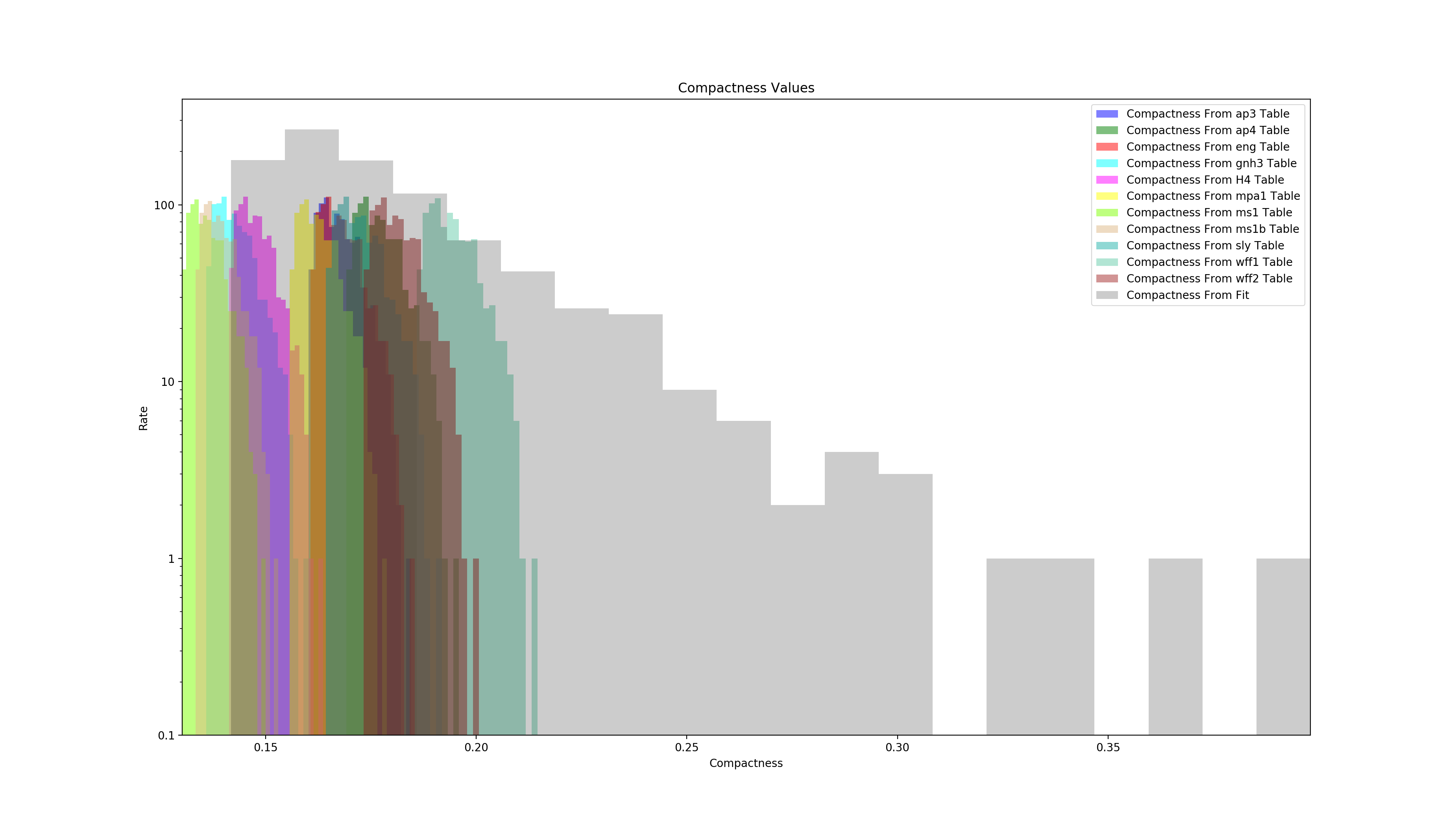
Calculating Compactness
Let’s Demonstrate some of the differences between calculating compactness from fit (i.e. being EOS agnostic) versus calculating it from a EOS.
>>> from gwemlightcurves.KNModels import KNTable
>>> from gwpy.table import EventTable
>>> from gwpy.plotter import EventTablePlot
>>> t = KNTable.read_samples('posterior_samples.dat')
>>> t = t.calc_tidal_lambda(remove_negative_lambda=True)
>>> plot = EventTablePlot(figsize=(18.5, 10.5))
>>> ax = plot.gca()
>>> EOS = ['ap3', 'ap4', 'eng', 'gnh3', 'H4', 'mpa1', 'ms1', 'ms1b', 'sly', 'wff1', 'wff2']
>>> Color = ['blue', 'green', 'red', 'cyan', 'magenta', 'yellow', 'chartreuse', 'burlywood', 'lightseagreen', 'mediumaquamarine', 'brown']
>>> EOS_Color = dict(zip(EOS, Color))
>>> for eos in EOS:
>>>     t_radius = t.calc_radius(EOS=eos, TOV='Monica')
>>>     t_radius_compact = t_radius.calc_compactness()
>>>     t_radius_compact = EventTable(t_radius_compact)
>>>     ax.hist(t_radius_compact['c1'], log=True, bins=20, alpha=0.5, histtype='stepfilled', label='Compactness From {0} Table'.format(eos), color=EOS_Color[eos])
>>> t_comp_fit = t.calc_compactness(fit=True)
>>> ax.hist(t_comp_fit['c1'], log=True, bins=20, alpha=0.2, histtype='stepfilled', label='Compactness From Fit', color='black')
>>> ax.set_xlabel('Compactness')
>>> ax.set_ylabel('Rate')
>>> ax.set_title('Compactness Values')
>>> plot.add_legend()
>>> ax.autoscale(axis='x', tight=True)
>>> plot.show()
(Source code, png, hires.png, pdf)

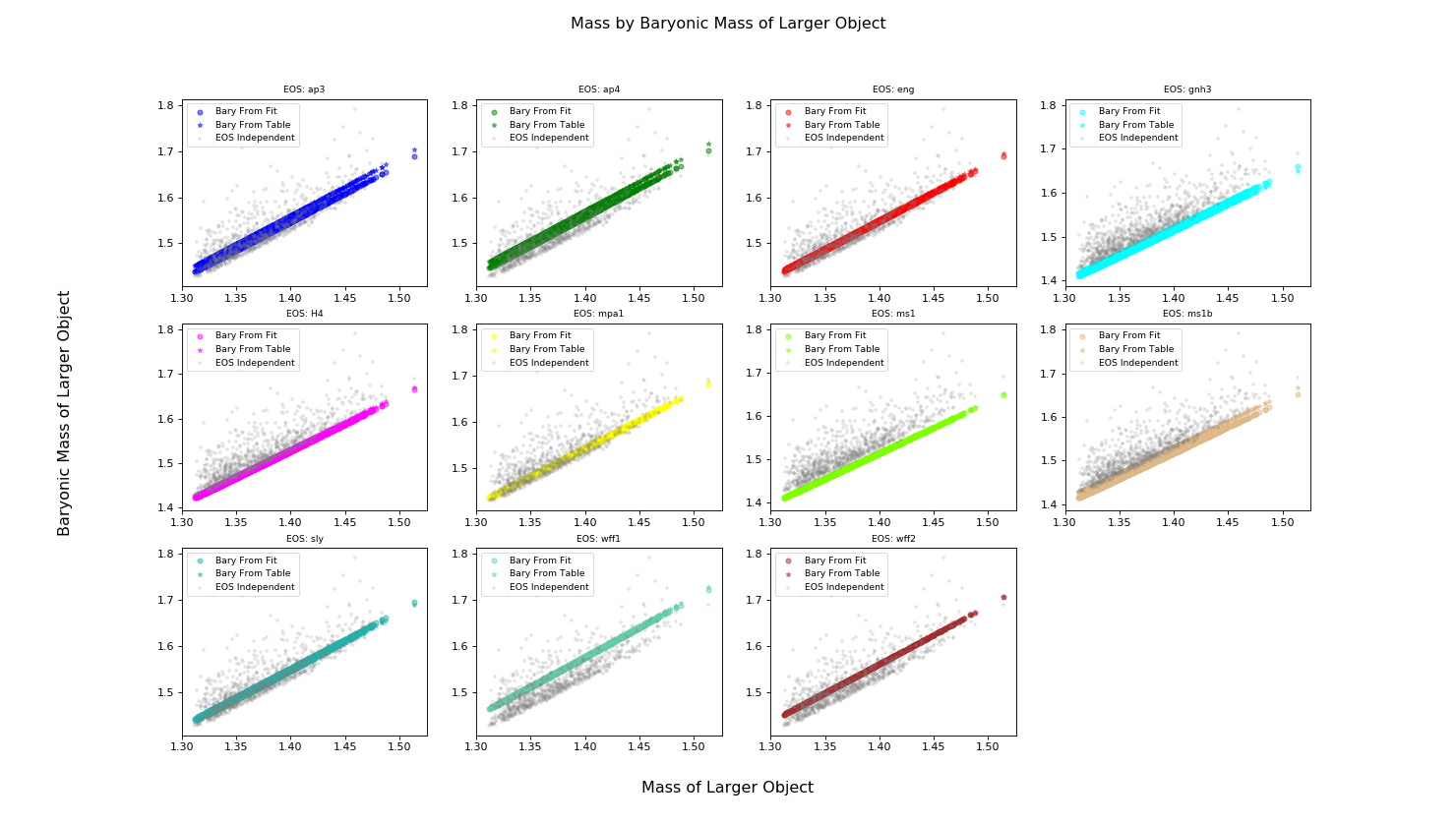
Calculating Baryonic Mass
Let’s demonstrate some of the differences between calculating the baryonic_mass from fit versus calculating it from an EOS table.
>>> from gwemlightcurves.KNModels import KNTable
>>> from gwpy.table import EventTable
>>> from gwpy.plotter import EventTablePlot
>>> t = KNTable.read_samples('posterior_samples.dat')
>>> t_indepedent = KNTable.read_samples('posterior_samples.dat')
>>> t = t.calc_tidal_lambda(remove_negative_lambda=True)
>>> t_indepedent = t_indepedent.calc_tidal_lambda(remove_negative_lambda=True)
>>> t = t.downsample(Nsamples=1000)
>>> t_indepedent = t_indepedent.downsample(Nsamples=1000)
>>> plot = EventTablePlot(figsize=(18.5, 10.5))
>>> EOS = ['ap3', 'ap4', 'eng', 'gnh3', 'H4', 'mpa1', 'ms1', 'ms1b', 'sly', 'wff1', 'wff2']
>>> Color = ['blue', 'green', 'red', 'cyan', 'magenta', 'yellow', 'chartreuse', 'burlywood', 'lightseagreen', 'mediumaquamarine', 'brown']
>>> locations = [(3,4,1), (3,4,2), (3,4,3), (3,4,4), (3,4,5), (3,4,6), (3,4,7), (3,4,8), (3,4,9), (3,4,10), (3,4,11)]
>>> plot_location = dict(zip(EOS, locations))
>>> EOS_Color = dict(zip(EOS, Color))
>>> t_indepedent = t_indepedent.calc_compactness(fit=True)
>>> t_indepedent = t_indepedent.calc_baryonic_mass(EOS=None, TOV=None, fit=True)
>>> for eos in EOS:
>>>     ax = plot.add_subplot(plot_location[eos][0], plot_location[eos][1], plot_location[eos][2])
>>>     ax.set_title('EOS: {0}'.format(eos), fontsize='small')
>>>     for fit in [True, False]:
>>>         t_radius = t.calc_radius(EOS=eos, TOV='Monica')
>>>         t_radius_compact = t_radius.calc_compactness()
>>>         t_radius_compact_bary = t_radius_compact.calc_baryonic_mass(EOS=eos, TOV='Monica', fit=fit)
>>>         t_radius_compact_bary = EventTable(t_radius_compact_bary)
>>>         if fit:
>>>             plot.add_scatter(t_radius_compact_bary['m1'], t_radius_compact_bary['mb1'], label='Bary From Fit', alpha=0.5, color=EOS_Color[eos], ax=ax)
>>>         else:
>>>             plot.add_scatter(t_radius_compact_bary['m1'], t_radius_compact_bary['mb1'], label='Bary From Table', alpha=0.5, color=EOS_Color[eos], marker='*', ax=ax)
>>>     plot.add_scatter(t_indepedent['m1'], t_indepedent['mb1'], label='EOS Independent', alpha=0.2, color='grey', marker='+', ax=ax)
>>>     plot.add_legend(loc="upper left", fancybox=True, fontsize='small')
>>> plot.text(0.5, 0.04, 'Mass of Larger Object', ha='center', fontsize='x-large')
>>> plot.text(0.04, 0.5, 'Baryonic Mass of Larger Object', va='center', rotation='vertical', fontsize='x-large')
>>> plot.suptitle('Mass by Baryonic Mass of Larger Object', fontsize='x-large')
>>> plot.show()
(Source code, png, hires.png, pdf)
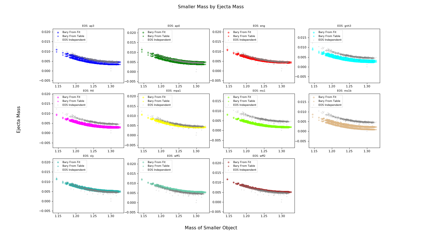
Calculating Ejecta Mass and Velocity of Ejecta
Now that we have compactness and the baryonic mass we can calculate Mass of the ejecta and the velocity of the ejecta using fits from Tim Dietrich and Maximiliano Ujevic
The dynamical ejecta mass fit formula can be found
https://arxiv.org/pdf/1612.03665.pdf#equation.3.1
and the constants are taken from
https://arxiv.org/pdf/1612.03665.pdf#equation.3.2
The method used to calculate in this repo is gwemlightcurves.EjectaFits.DiUj2017.calc_meje() and can be used as follows:
>>> from gwemlightcurves.EjectaFits.DiUj2017 import calc_meje
>>> from gwemlightcurves.KNModels import KNTable
>>> t = KNTable.read_samples('posterior_samples.dat')
>>> t = t.calc_tidal_lambda(remove_negative_lambda=True)
>>> t_sly_mon = t.calc_radius(EOS='sly', TOV='Monica')
>>> t_sly_mon = t_sly_mon.calc_compactness()
>>> t_sly_mon = t_sly_mon.calc_baryonic_mass(EOS='sly', TOV='Monica')
>>> t_sly_mon['mej'] = calc_meje(t_sly_mon['m1'], t_sly_mon['mb1'], t_sly_mon['c1'], t_sly_mon['m2'], t_sly_mon['mb2'], t_sly_mon['c2'])
The velocity of the ejecta mass fit can be found:
https://arxiv.org/pdf/1612.03665.pdf#equation.3.9
The method used to calculate in this repo is gwemlightcurves.EjectaFits.DiUj2017.calc_vej() and can be used as follows:
>>> from gwemlightcurves.EjectaFits.DiUj2017 import calc_vej
>>> t_sly_mon['mej'] = calc_vej(t_sly_mon['m1'], t_sly_mon['c1'], t_sly_mon['m2'], t_sly_mon['c2'])
>>> from gwemlightcurves.EjectaFits.DiUj2017 import calc_meje, calc_vej
>>> from gwemlightcurves.KNModels import KNTable
>>> from gwpy.table import EventTable
>>> from gwpy.plotter import EventTablePlot
>>> t = KNTable.read_samples('posterior_samples.dat')
>>> t_indepedent = KNTable.read_samples('posterior_samples.dat')
>>> t = t.calc_tidal_lambda(remove_negative_lambda=True)
>>> t_indepedent = t_indepedent.calc_tidal_lambda(remove_negative_lambda=True)
>>> t = t.downsample(Nsamples=1000)
>>> t_indepedent = t_indepedent.downsample(Nsamples=1000)
>>> plot = EventTablePlot(figsize=(18.5, 10.5))
>>> EOS = ['ap3', 'ap4', 'eng', 'gnh3', 'H4', 'mpa1', 'ms1', 'ms1b', 'sly', 'wff1', 'wff2']
>>> Color = ['blue', 'green', 'red', 'cyan', 'magenta', 'yellow', 'chartreuse', 'burlywood', 'lightseagreen', 'mediumaquamarine', 'brown']
>>> locations = [(3,4,1), (3,4,2), (3,4,3), (3,4,4), (3,4,5), (3,4,6), (3,4,7), (3,4,8), (3,4,9), (3,4,10), (3,4,11)]
>>> plot_location = dict(zip(EOS, locations))
>>> EOS_Color = dict(zip(EOS, Color))
>>> t_indepedent = t_indepedent.calc_compactness(fit=True)
>>> t_indepedent = t_indepedent.calc_baryonic_mass(EOS=None, TOV=None, fit=True)
>>> t_indepedent['mej'] = calc_meje(t_indepedent['m1'], t_indepedent['mb1'], t_indepedent['c1'], t_indepedent['m2'], t_indepedent['mb2'], t_indepedent['c2'])
>>> for eos in EOS:
>>>     ax = plot.add_subplot(plot_location[eos][0], plot_location[eos][1], plot_location[eos][2])
>>>     ax.set_title('EOS: {0}'.format(eos), fontsize='small')
>>>     for fit in [True, False]:
>>>         t_radius = t.calc_radius(EOS=eos, TOV='Monica')
>>>         t_radius_compact = t_radius.calc_compactness()
>>>         t_radius_compact_bary = t_radius_compact.calc_baryonic_mass(EOS=eos, TOV='Monica', fit=fit)
>>>         t_radius_compact_bary['mej'] = calc_meje(t_radius_compact_bary['m1'], t_radius_compact_bary['mb1'], t_radius_compact_bary['c1'], t_radius_compact_bary['m2'], t_radius_compact_bary['mb2'], t_radius_compact_bary['c2'])
>>>         t_radius_compact_bary = EventTable(t_radius_compact_bary)
>>>         if fit:
>>>             plot.add_scatter(t_radius_compact_bary['m2'], t_radius_compact_bary['mej'], label='Bary From Fit', alpha=0.5, color=EOS_Color[eos], ax=ax)
>>>         else:
>>>             plot.add_scatter(t_radius_compact_bary['m2'], t_radius_compact_bary['mej'], label='Bary From Table', alpha=0.5, color=EOS_Color[eos], marker='*', ax=ax)
>>>     plot.add_scatter(t_indepedent['m2'], t_indepedent['mej'], label='EOS Independent', alpha=0.2, color='grey', marker='+', ax=ax)
>>>     plot.add_legend(loc="upper left", fancybox=True, fontsize='small')
>>> plot.text(0.5, 0.04, 'Mass of Smaller Object', ha='center', fontsize='x-large')
>>> plot.text(0.04, 0.5, 'Ejecta Mass', va='center', rotation='vertical', fontsize='x-large')
>>> plot.suptitle('Smaller Mass by Ejecta Mass', fontsize='x-large')
>>> plot.show()
(Source code, png, hires.png, pdf)

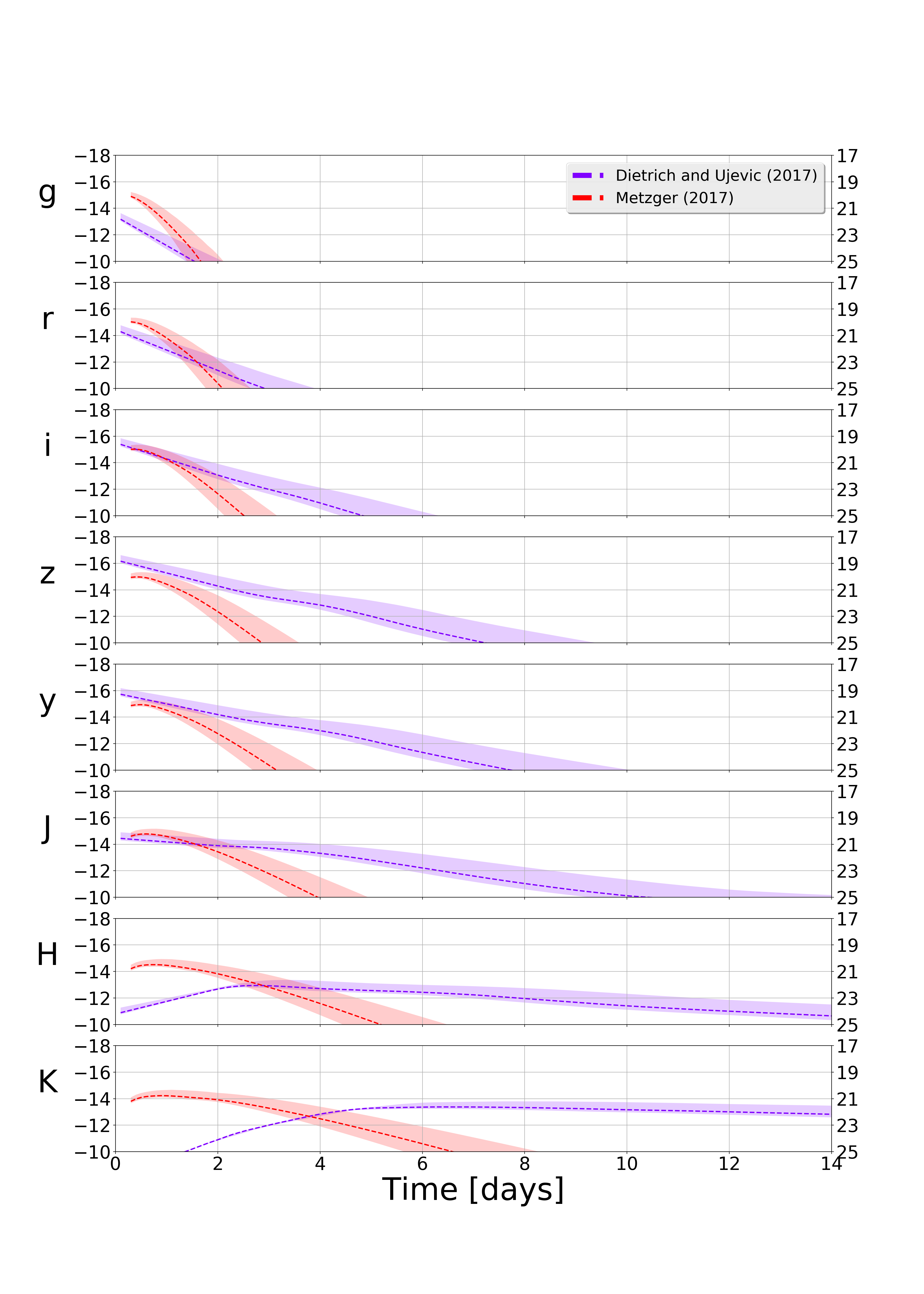
Generating Light Curves
Finally, let’s calculate a lightcurve being EOS agnostic. That is, we calculate both the compactness and baryonic masses from fits. Also let us look at a Metzer 2017 and DiUj2017 models. In order to take a set of samples and calculate the light curves that would result from a realization of each sample you can you the model which takes as inputs the string name of the model and the table of samples containing at minimum compactness and baryonic mass (it can clauclate mass ejecta and velocity of ejecta on the fly)
>>> from gwemlightcurves.KNModels import KNTable
>>> from gwemlightcurves import lightcurve_utils
>>> t = KNTable.read_samples('posterior_samples.dat')
>>> t = t.calc_tidal_lambda(remove_negative_lambda=True)
>>> t = t.calc_compactness(fit=True)
>>> t = t.calc_baryonic_mass(EOS=None, TOV=None, fit=True)
>>> t = t.downsample(Nsamples=100)
>>> tini = 0.1; tmax = 50.0; dt = 0.1; vmin = 0.02; th = 0.2; ph = 3.14; kappa = 1.0; eps = 1.58*(10**10); alp = 1.2; eth = 0.5; flgbct = 1; beta = 3.0; kappa_r = 1.0; slope_r = -1.2; theta_r = 0.0; Ye = 0.3
>>> t['tini'] = tini; t['tmax'] = tmax; t['dt'] = dt; t['vmin'] = vmin; t['th'] = th; t['ph'] = ph; t['kappa'] = kappa; t['eps'] = eps; t['alp'] = alp; t['eth'] = eth; t['flgbct'] = flgbct; t['beta'] = beta; t['kappa_r'] = kappa_r; t['slope_r'] = slope_r; t['theta_r'] = theta_r; t['Ye'] = Ye
>>> # Create dict of tables for the various models, calculating mass ejecta velocity of ejecta and the lightcurve from the model
>>> models = ["DiUj2017","Me2017"]
>>> model_tables = {}
>>> for model in models:
>>>     model_tables[model] = KNTable.model(model, t)
>>> # Now we need to do some interpolation
>>> for model in models:
>>>    model_tables[model] = lightcurve_utils.calc_peak_mags(model_tables[model])
>>>    model_tables[model] = lightcurve_utils.interpolate_mags_lbol(model_tables[model])
>>> distance = 100 #Mpc
>>> plot = KNTable.plot_mag_panels(model_tables, distance=distance)
>>> plot.show()
(Source code, png, hires.png, pdf)
